Wikipedia: https://en.wikipedia.org/wiki/Entropy_%28information_theory%29
Entropy
Information entropy measures the unpredictability. Depending on the probability distribution generating the events, the entropy measures how well we can predict the outcome of a sample.
Formally, entropy (

![H(X) = E[-log(p(X))]](https://s0.wp.com/latex.php?latex=H%28X%29+%3D+E%5B-log%28p%28X%29%29%5D++++&bg=ffffff&fg=333333&s=0&c=20201002)
and for a discrete domain:

For example, for a fair coin, the probability of getting heads P(head) is equal to the probability of getting tails P(tail), both being equal to 0.5. Thus, the entropy of the fair coin would be 1.0. Another example, a fair dice would have a probability of 1/6 for each of its sides, thus giving an entropy of 2.585.
The entropy of a distribution can thus be seen as the number of bits required to encode a single sample drawn from the distribution. For a (fair) coin toss, this is 1 bit, for a dice toss, it’s just under 3 bits.
Cross-entropy
Given the true distribution 

![H(p,q) = E_{p(X)} [-log(q(X))]](https://s0.wp.com/latex.php?latex=H%28p%2Cq%29+%3D+E_%7Bp%28X%29%7D+%5B-log%28q%28X%29%29%5D++++&bg=ffffff&fg=333333&s=0&c=20201002)
For a discrete domain:

Thus, cross-entropy measures the efficiency of the optimal encoding for the approximating distribution 

For example, if our true distribution models a fair dice and our approximating distribution assigns probability 0.5 to one side and 0.1 to each of the five other sides, the cross-entropy is

which is higher than a perfectly matching approximating distribution, in which case the cross-entropy would equal the entropy of
Kullback-Leibler divergence
(A.k.a. information gain.)
KL divergence 
In term of entropies defined earlier:

For discrete domains:
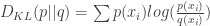
The more the approximating distribution
KL divergence can not be negative (at least 0, when 
For our dice example, the KL divergence would be 0.3, the difference in bits required to encode a sample from true distribution
Perplexity
Perplexity of a probability distribution

with 
Illustratory, perplexity measures the predictability of some distribution, giving the number of possible outcomes of an equally (un)predictable distribution if each of those outcomes was given the same probability.
For example, if some distribution
Perplexity of a model
Consider a distribution

where 
